Regression Models: Speed

library(tidyverse)
library(FITfileR)
library(dplyr)
library(patchwork)
library(leaflet)
library(modelr)

training_raw <- read_csv("activities/activities.csv") %>% 
  janitor::clean_names()

training_summary = 
  training_raw %>% 
  filter(activity_type == "Run") %>%
  select(activity_id, activity_date, activity_name, activity_description, elapsed_time_6, distance_7, max_heart_rate_8, relative_effort_9, max_speed, average_speed, elevation_gain, elevation_loss, max_grade, average_grade, max_cadence, average_cadence, average_heart_rate, calories, weather_temperature, dewpoint, humidity, wind_speed) %>%
  filter(activity_id >= 6910869137) %>%
  separate(activity_date, c("month_date", "year", "time"), sep = ", ") %>%
  mutate(
    date = str_c(month_date, year, sep = " "),
    date = as.Date(date, format = "%b%d%Y")
  ) %>%
  select(-month_date, -year) %>%
  mutate(
    elapsed_time_min = elapsed_time_6 / 60,
    distance_km = distance_7,
    max_heart_rate = max_heart_rate_8,
    relative_effort = relative_effort_9
  ) %>%
  select(-elapsed_time_6, -distance_7, -max_heart_rate_8, -relative_effort_9)
activity_summaries =
  training_summary %>%
  select(activity_id, date, time, activity_name, activity_description)

tidy_training = 
  training_summary %>%
  select(-activity_name, -activity_description) %>%
  select(activity_id, date, time, distance_km, elapsed_time_min, max_speed, average_speed, max_heart_rate, average_heart_rate, relative_effort, everything()) %>% 
  filter(date != "2022-03-31", 
         date != "2022-04-03")

Based on Emma’s recount of personal experience, she perceives environmental factors to be significant predictors of her performance. More specifically, weather conditions such as temperature, humidity, dewpoint, and windspeed affect Emma’s perceived running experience. Additionally, due to the irregular environmental conditions on race day, we generated several models to investigate which environmental factors would be best predictors for Emma’s performance. We hypothesize that Emma’s average speed is dependent on temperature. To test this hypothesis, we built the following models:

Average speed vs temperature
Average speed vs dewpoint
Average speed vs humidity
Average speed vs elevation gain and wind speed, and all interactions
Average speed vs temperature and dewpoint, and all interactions

fit1 = lm(average_speed ~ weather_temperature, data = tidy_training)
fit2 = lm(average_speed ~ dewpoint, data = tidy_training)
fit3 = lm(average_speed ~ humidity, data = tidy_training)
fit4 = lm(average_speed ~ (elevation_gain + wind_speed)^3, data = tidy_training)
fit5 = lm(average_speed ~ (weather_temperature + dewpoint)^3, data = tidy_training)

Cross-Validation: Speed

We can now perform a comparison between the five models in terms of cross-validated prediction error. To do this, we first create a cross-validation data frame cv_df. Contained within cv_df is 2 side-by-side list columns with the testing and training data split pairs, with a corresponding ID number for each pair. Since we are able to apply resample objects directly into lm functions, we can skip the extra step of converting the testing and training data into tibbles. Next, we apply the map function to map each regression model to the training data. Finally, we can compute the root mean squared errors (RMSEs) for each model by applying the map2_dbl function to the testing data.

cv_df = 
  crossv_mc(tidy_training, 100)

cv_df = cv_df %>% 
  mutate(
    mod1 = map(.x = train, ~lm(average_speed ~ weather_temperature, data = .x)), 
    mod2 = map(.x = train, ~lm(average_speed ~ dewpoint, data = .x)), 
    mod3 = map(.x = train, ~lm(average_speed ~ humidity, data = .x)), 
    mod4 = map(.x = train, ~lm(average_speed ~ (elevation_gain + wind_speed)^3, data = .x)),
    mod5 = map(.x = train, ~lm(average_speed ~ (weather_temperature + dewpoint)^3, data = .x))) %>% 
  mutate(
    rmse_mod1 = map2_dbl(.x = mod1, .y = test, ~rmse(model = .x, data = .y)), 
    rmse_mod2 = map2_dbl(.x = mod2, .y = test, ~rmse(model = .x, data = .y)), 
    rmse_mod3 = map2_dbl(.x = mod3, .y = test, ~rmse(model = .x, data = .y)),
    rmse_mod4 = map2_dbl(.x = mod4, .y = test, ~rmse(model = .x, data = .y)),
    rmse_mod5 = map2_dbl(.x = mod5, .y = test, ~rmse(model = .x, data = .y)))

cv_df %>% 
  select(starts_with("rmse")) %>% 
  pivot_longer(
    everything(), 
    names_to = "model", 
    values_to = "rmse", 
    names_prefix = "rmse_") %>% 
  ggplot(aes(x = model, y = rmse, color = c("#FFA500"))) +
  geom_boxplot(color = c("#FFA500")) + 
  labs(
    title = "Root Mean Squared Errors Distributions for Emma's Average Speed", 
    x = "Fitted Model", 
    y = "RMSE")  + 
  theme(axis.line = element_line(color = "grey"), 
        panel.background = element_blank(), 
        legend.position = "none", 
        panel.grid.major = element_line(color = "light grey", linetype = "dashed"),
        plot.title = element_text(hjust = 0.5)) +
  scale_x_discrete(labels = c("mod1" = "Temperature Model", 
                              "mod2" = "Dewpoint Model", 
                              "mod3" = "Humidity Model",
                              "mod4" = "Elevation, Wind, \n Interactions",
                              "mod5" = "Temperature, Dewpoint, \n Interactions"))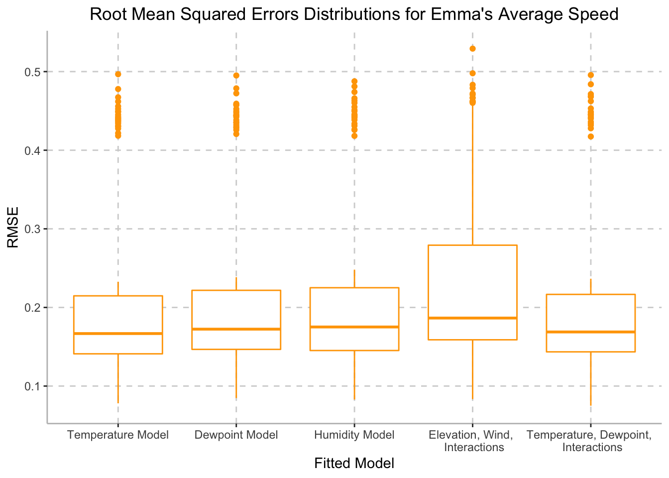

summary(fit1) %>% 
  broom::tidy() %>% 
  filter(term == "weather_temperature") %>% 
  mutate(
    lower_ci = exp(estimate - 1.96*std.error),
    upper_ci = exp(estimate + 1.96*std.error)
  ) %>% 
  select(term, estimate, lower_ci, upper_ci, p.value) %>% 
  knitr::kable(digits = 3, 
               col.names = c("Term", "Estimate", "Lower CI", "Upper CI", "P-value"))

Term	Estimate	Lower CI	Upper CI	P-value
weather_temperature	0.011	1.001	1.021	0.031

Based on the distributions depicted above, we can conclude that the model with temperature is able to generate better predictions than the other models with environmental factors. The p-value for this model is 0.03101. As it is below the significance level of 0.05, we can conclude that this model is a good predictor for average speed.